What is Image Segmentation with Deep Learning?

Deep learning can perform many of the same operations as conventional image processing. This is also true for segmentation. This article examines why segmentation is important and where segmentation by deep learning is preferable to classic image processing approaches.

Segmentation is different from classification or detection. Classification tells us if a specific object is in the image but not where it is or how many copies of it there are. Detection tells us where an object is in an image by drawing a box around each object’s location. Segmentation goes further by labeling each pixel in the image that belongs to an object. Segments make subsequent image processing easier or, in some cases, even possible. 

The results of segmentation are regions or pixels usually labeled with a value from 0 to n-1. For display, the segmented regions are presented as different colors.

Classic segmentation is the process of finding connected regions of pixels that share a common characteristic such as brightness, texture, or color. It operates at the pixel level.  A big challenge in classic segmentation is to define what constitutes a similarity between adjacent pixels or regions.

Deep learning segmentation goes further. It handles variations in size, shape, color, and shading as well as combinations of disparate parts by segmenting learned objects.

Related: Understanding Image Segmentation Basics-Part 1

Where is Image Segmentation Used?

Image segmentation is used in many types of vision applications including:

• Object recognition: Making recognition of individual objects practical.
• Surveillance: Recognizing objects in video feeds to enhance security.
• Tumor detection: Identifying potential tumors in X-ray, CT, and MRI scans.
• Organ segmentation: Identifying different organs in X-ray, CT, and MRI scans.
• Road scene analysis: Identifying and classifying different objects on or near the road.
• Quality assurance: Identifying potential defects or irregularities in products.
• Agriculture:  Identifying individual plants, fruit as well as weeds.
• AR and VR: Recognizing and interacting with real-world objects.
• Background removal: Removing or replacing the background during the photo editing process.
• Separate foreground and background: Enhancing the photo and video editing process.
• Land cover classification: Identifying surface components on land visible in satellite images.
• Environmental monitoring: Tracking changes in the ecosystem.
• Facial recognition: Extracting facial features to enable recognition.
• Navigation: Making terrain analysis practical and aiding in obstacle detection.
• Gesture recognition: Identifying body parts and enabling analysis of their movement.

What are the Shortcomings of Classic Image Segmentation Techniques?

Classic image segmentation uses either pixel similarity—how similar is a pixel to its neighbors—to form clusters or it uses discontinuity—how different is a pixel from its neighbors—to detect edges.¹ 

Classic segmentation fails when a single object may have disparate parts since the segmentation process has no semantic understanding.  For example, a screwdriver has a blade and a handle. These two parts will normally appear different in an image and have no uniformly common pixel characteristic.

Another example would be an application that needs to segment strawberries in an image. Dep learning can be trained on strawberries of different sizes, shapes, colors, and shading, allowing the application to segment them. But classic techniques relying only on amplitude or boundaries of a specific template (shape) will not work in this scenario.

Finally, classic segmentation often handles only one segmentation condition (e.g., a single threshold).  Deep learning segmentation can be trained to segment many different objects simultaneously.

Related: Understanding Image Segmentation Basics-Part 2

Segmentation with deep learning can handle objects with multiple parts including objects that are of variable shape, size, and color.  Deep learning segmentation handles complex scenes or changing object characteristics such as plants in agriculture or tumors in medical imaging.  With deep learning, segmentation can be trained to adapt to these different conditions.

What Are the Three Types of Segmentation?

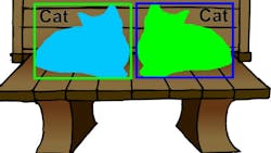
Segmentation can be differentiated from simple classification.  For example, a simple classifier trained to recognize a cat will give the same output “cat” for each of the two images below. (See Figure 1 and Figure 2.)

Semantic Segmentation

Segmentation of an image at the pixel level identifies all pixels having a desired characteristic. It does not determine the size or number of segmented regions.  For example, if Figure 2 above was segmented, the result would be as shown in Figure 3 where all pixels belonging to class “cat” are labeled the same without regard to the number of cats in the image.

Instance Segmentation

Instance segmentation identifies pixels belonging to each instance of a class.  However, it does not distinguish between the individual instances.  In Figure 4, each instance of a cat is identified but there is no indication that there are two cats.

Panoptic Segmentation

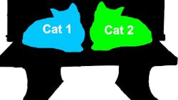
Panoptic segmentation combines semantic and instance segmentation to identify each instance of a segmented object in an image as shown in Figure 5 where the two cats are segmented and identified as separate instances.

How Does Deep Learning Segmentation Work?

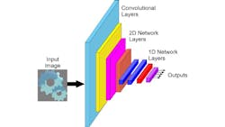
To understand deep learning segmentation, it’s best to start with a review of convolutional neural networks for classification.  A traditional convolutional neural network used for classification consists of a series of layers.  Each layer can be a convolutional layer, a pooling layer, or a fully connected layer.

Pooling layers reduce the dimensionality of the data, allowing generalization and data reduction to speed up processing.  Pooling also makes the network less sensitive to any feature’s location in the image.  Again, each cell takes its inputs from a specific array of cells in the preceding layer.  The most common pooling function is the maximum value in the input array of cells, although other operations, such as averaging, are possible.

In fully connected layers, each cell takes its inputs from all cells in the preceding layers. Each cell in the fully connected layer has as many weights as there are cells in the previous layer. The number of weights for a fully connected layer is the product of the number of cells in the two layers. Fully connected layers are often shown as 1D layers since the output of a classifier is a vector representing classes.  However, since every cell in the layer is connected with weights to every cell in the preceding layer, a fully connected layer has no inherent dimensionality.

Related: Understanding Region-based Segmentation

There are many different networks configured for classification and they often differ in the number and arrangement of the layers.

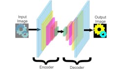
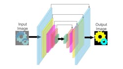
Deep learning segmentation uses a structure resembling the classification network in an encoder-decoder arrangement (see Figure 7).  There is an encoder that looks a lot like the classification network except that it doesn’t get reduced to an array of discrete outputs.

The decoder resembles a backward classification network starting from smaller layers and working up to a layer the size of an image.  It consists of fully connected layers, and they are one of two types:

• Upsampling layers that replace the pooling layers of the encoder to increase, rather than decrease, the size of the result.
• Transpose convolutional layers that not only increase the size of the result but also provide an increase in dimensionality.

The connection between the encoder and decoder, as shown in Figure 7 above, is called the bridge or bottleneck.  While this encoder-decoder network can perform segmentation at some level, it loses so much detail at the bridge that the segmentation at the pixel level is very coarse at best.  

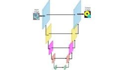
The most popular modification to the simple encoder-decoder network is to have the outputs of the encoder layers serve as additional inputs to the corresponding decoder layer as shown in Figure 8 above.  Diagrammed differently as Figure 9 below, this network is known as the U-Net.  The U-Net network preserves pixel information from the input of the encoder through the output of the decoder.

Researchers have developed a number of additional network architectures to help solve segmentation such as U-Net+ and V-Net, both of which incorporate more layers.

 How Does Training the Encoder-Decoder Work?

The typical training for segmentation starts by training only the encoder as a classifier using labeled images; the labels identifying the objects in the image.  The encoder learns to recognize the classes of objects that it should enable for segmentation. The encoder must be trained to a high level of accuracy for reliable segmentation.

Following the encoder training, the decoder part is trained using training images that have been annotated by outlining or shading the objects’ pixels needing segmentation—that is, they are manually segmented.

Training requires feedback.  For the encoder, the feedback is the error between its outputs and the labels.  For the decoder, it is based upon how well each of the encoder’s output pixels match the manually labeled pixels.

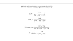
The quality of segmentation is based on four pixel counts: 

• True positive (TP), representing the pixels labeled as part of the object and belonging to the object.
• True negative, (TN), representing pixels that are labeled as not part of the object and belonging to the background or some other object
• False positive (FP), representing pixels labeled as part of the object that do not belong to the object
• False negative (FN), representing pixels that are labeled as not part of the object but are actually part of the object.

Given these four counts, there are many metrics in use for determining the quality of the segmentation. One is the Intersection of Union (IoU) or Jaccard index.  Another is the Dice similarity coefficient (DSC) or F1 score.  Still other metrics measure the accuracy and the precision of the training.

Conclusion

In establishing deep learning segmentation, the number of training images needed as well as the effort to label and annotate those images should not be underestimated.

However, deep learning segmentation will succeed with low-quality images or content that is intractable with classic image segmentation algorithms. Still, the performance of deep learning segmentation will be highest when used with high quality images having good contrast and low noise.

Segmentation using deep learning is an available tool that extends machine vision and computer vision well beyond classic segmentation techniques.  Where classic techniques work reliably, they are most likely preferable to using DL.  When the classical segmentation techniques are unreliable, segmentation with DL becomes a powerful tool to solve a wide class of applications.

 References

1. Jasim, W. and Mohammed, R.; “A Survey on Segmentation Techniques for Image Processing”, 2020; https://ijeee.edu.iq/Papers/Vol17-Issue2/1570736047.pdf